Benchmarking Tasks

Benchmark Divisions

There are two divisions of benchmarking, the closed one which is restrictive to allow fair comparisons of specific training algorithms and systems, and the open divisions, which allows users to run their own models and code while still providing a reasonably fair comparison.

Closed Division

The Closed Division encompasses several subcategories to compare different dimensions of distributed machine learning. We provide precise reference implementations of each algorithm, including the communication patterns, such that they can be implemented strictly comparable between different hardware and software frameworks.

The two basic metrics for comparison are Accuracy after Time and Time to Accuracy (where accuracy will be test and/or training accuracy)

Variable dimensions in this category include:

• Algorithm - limited number of prescribed standard algorithms, according to strict reference implementations provided
• Hardware - GPU - CPU(s) - Memory
• Scalability - Number of workers
• Network - Impact of bandwidth and latency

Accuracy after Time

The system has a certain amount ot time for training (2 hours) and at the end, the accuracy of the final model is evaluated. The higher the better

Time to Accuracy

A certain accuracy, e.g. 97% is defined for a task and the training time of the system until that accuracy is reached is measured. The shorter the better.

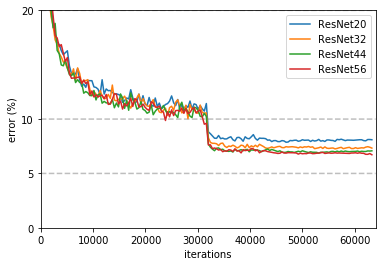
Here is a plot of validation error training iterations for ResNet on `CIFAR-10<http://www.cs.toronto.edu/~kriz/cifar.html>`_ using the settings from Deep Residual Learning for Image Recognition.

Open Division

The Open Division allows you to implement your own algorithms and training tricks and compare them to other implementations. There’s little limit to what can be changed by you and as such, it is up to you to make sure that comparisons are fair.

In this division, mlbench merely provides a platform to easily perform and measure distributed machine learning experiments in a standardized way.

Benchmark Task Descriptions

We here provide precise descriptions of the official benchmark tasks. The task are selected to be representative of relevant machine learning workloads in both industry and in the academic community. The main goal here is a fair, reproducible and precise comparison of most state-of-the-art algorithms, frameworks, and hardware.

For each task, we provide a reference implementation, as well as benchmark metrics and results for different systems.

1a. Image Classification (ResNet, CIFAR-10)

Image classification is one of the most important problems in computer vision and a classic example of supervised machine learning.

1. Model

   We benchmark two model architectures of Deep Residual Networks (ResNets) based on prior work by He et al. The first model (m1) is based on the ResNets defined in this paper. The second version (m2) is based on the ResNets defined here. For each version we have the network implementations with 20, 32, 44, and 56 layers.

   TODO: only benchmark two most common architectures say (can support more, but they are not part of the official benchmark task)

2. Dataset

   The CIFAR-10 dataset containing a set of images used to train machine learning and computer vision models. It contains 60,000 32x32 color images in 10 different classes, with 6000 images per class. The 10 different classes represent airplanes, cars, birds, cats, deer, dogs, frogs, horses, ships, and trucks.

   The train / test split as provided in the dataset is used. The test dataset contains 10,000 imagest with exactly 1000 randomly-selected images per each class. The rest 50,000 images are training samples.

3. Training Algorithm

   We use standard synchronous SGD as the optimizer (that is distributed mini-batch SGD with synchronous all-reduce communication after each mini-batch).

   • number of machines \(k\): 2, 4, 8, 16, 32
   • minibatch size per worker \(b\): 32
   • maximum epochs: 164
   • learning rate
     • learning rate per sample \(\eta\) : 0.1 / 256
     • decay: similar to Deep Residual Learning for Image Recognition, we reduce learning rate by 1/10 at the 82-th and 109-th epoch.
     • scaling and warmup: apply linear scaling rule mentioned in goyal2017accurate. The learning rate per worker is scaled from \(\eta \times b\) to \(\eta \times b \times k\) within the first 5 epochs.
   • momentum: 0.9
   • nesterov: True
   • weight decay: 0.0001

   Besides, in each round workers access disjoint set of datapoints.

Implementation details:

1. Data Preprocessing

   We followed the same approach as mentioned here.

2. Selection of Framework & Systems

   While our initial reference implementation is currently PyTorch, we will aim to provide the same algorithm in more frameworks very soon, starting with Tensorflow. For the systems, kubernetes allows easy transferability of our code. While initial results reported are from google kubernetes engine, AWS will be supported very soon.

3. Environments for Scaling Task

   For the scaling task, we use n1-standard-4 type instances with 50GB disk size. There is only one worker per node; each worker uses 2.5 cpus. The bandwidth between two nodes is around 7.5Gbit/s. Openmpi is used for communication. No accelerators are used for this task.

Results

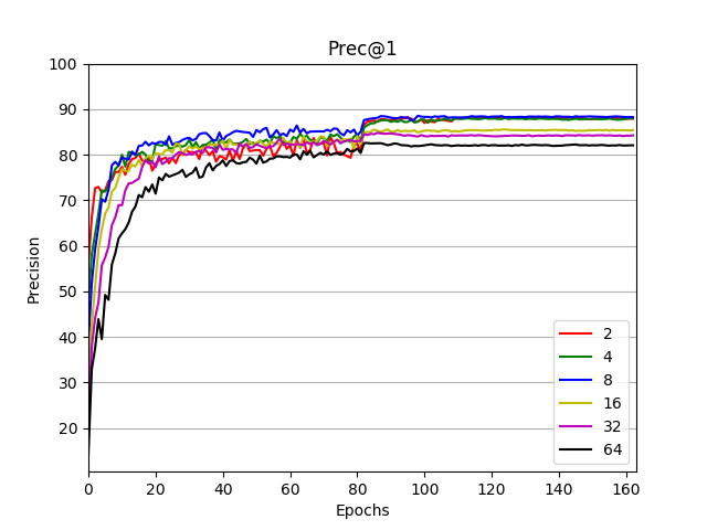
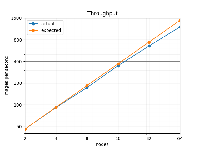
Here we present the results for scaling task.

• The left figure is an epoch to accuracy curve. For 2, 4, 8 nodes, scaling the size of cluster gives same accuracy. For 16 or more nodes, the accuracy gradually drops.
• The right hand side compares expected throughput with the actual throughput. From the figure, we can see the actual throughput is marginally below ideal scaling.

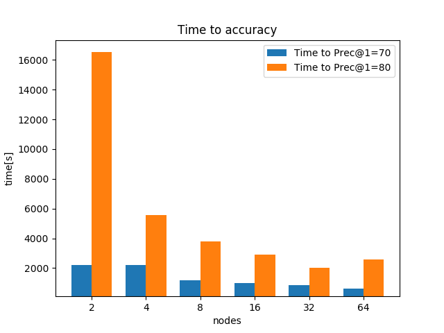
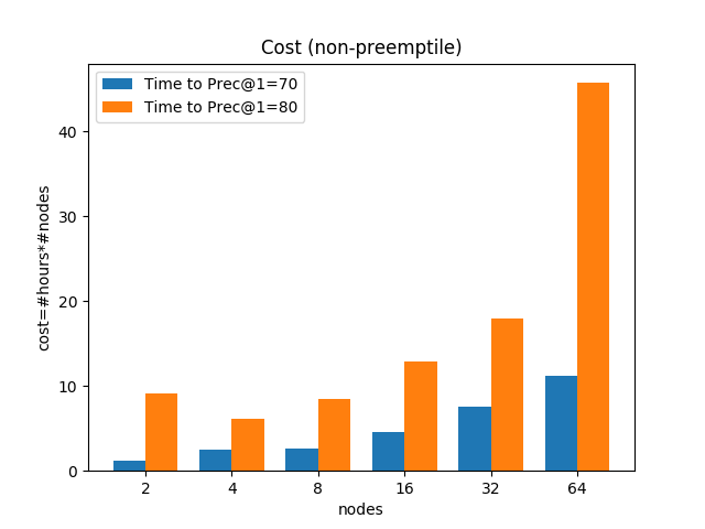
• The left figure hand side figure compares the time to 70% and 80% accuracy for different number of nodes. 70% accuracy is easy to reach for all of the tests and the time-to-accuracy decreases with the number of nodes. For time-to-80%-accuracy, however, it spends more time on 64 nodes rather than 32 nodes.
• The right figure compares the cost of experiment. Note that a regular n1-standard-4 instance costs $0.1900 per hour and a preemptible one costs only $0.04. For experiments with 16 nodes or more, the task finishes with 24 hours and thus we can use preemptible instance. The cost can be reduced correspondingly.

1b. Image Classification (ResNet, ImageNet)

TODO (again synchr SGD as main baseline)

2. Linear Learning (Generalized Linear Models for Regression and Classification)

TODO (more data intensive compared to deep learning. again synchr SGD as main baseline)

[goyal2017accurate]

Goyal, Priya, et al. Accurate, large minibatch SGD: training imagenet in 1 hour.